Encapsulated Pumped Storage, Series 2, Part 2: Hydrodynamics

In the last post, I described a fast, inexpensive way of building evaporation-proof water storage on gently sloping terrain. One risk of building a pumped storage solution around this method is that the penstocks will tend to be long, compared to more traditional hydroelectric systems.

Penstocks

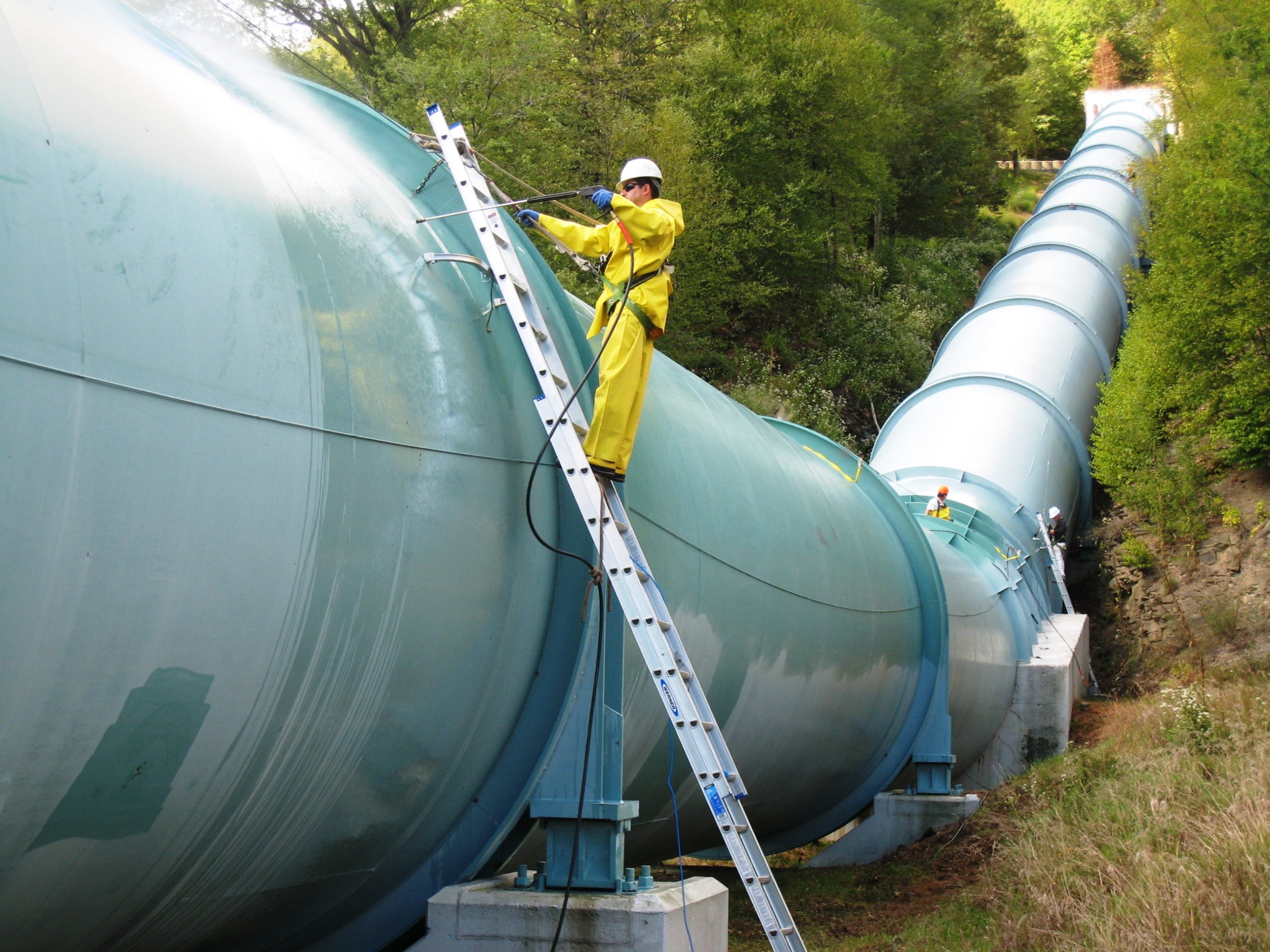
Penstocks are the large pipes (one or more) that carry water between the upper storage area and the powerhouse. They must be very strong because the peak pressure of the system is realized at the bottom of the penstock, where it enters the turbine. The combined requirements of strength and size make the penstocks a significant contributor to the overall system cost. Headraces and tailraces (defined in the previous post) don’t have to withstand the high water pressures that the penstocks do, which should help limit the cost of those components.

In a traditional hydropower plant where a river is dammed to create a reservoir, penstocks can be relatively short (not much more than the thickness of the dam itself). Closed-loop pumped storage systems (such as EPS) generally need longer penstocks, because the elevation difference is created by natural terrain, rather than a dam. (We could minimize penstock length by aiming the penstocks vertically down from the upper storage area, but this would typically require placing the powerhouse in a location deep within the earth, resulting in higher construction costs and a much longer time from the start of construction until the site comes online.) The more gradual the average slope between upper and lower storage, the longer the penstocks need to be. This will make them more expensive and less hydrodynamically efficient. At the same time, there are sites that are very appealing aside from requiring long penstocks; so we need to quantify how long penstocks can be before the costs outweigh the benefits.

Water flowing in a container, such as a pipe, is constantly losing some of its energy to friction against the container walls, and to internal friction against itself. This lost energy reduces how much energy a pumped storage system can store and later retrieve. So it’s a key design goal to minimize these losses.

This trades off against cost. The simplest way to reduce energy loss in a pipe, assuming it can’t be made shorter, is to make it larger in diameter, but larger pipes cost more. So it’s an optimization problem: we want to maximize the amount of stored energy we can get out of the system, per dollar spent building it.

Scenarios

I’ll look at penstock losses in the context of high, medium, and low head (1,000 m, 670 m, and 362 m)—representing three actual sites of interest for EPS. The cross-section drawing above is of the medium-head scenario, which looks like this as a Google Earth profile:

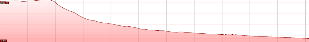
This image has been scaled to show true elevation (horizontal and vertical scale are the same). The elevation at the far left is 2,020 meters (6,630 ft), and at the far right, it’s about 1,350 meters (4430 ft). So the usable vertical drop is 670 meters (2,200 ft). The full horizontal span is about 5.5 km (about 18,000 feet, or 3.4 miles).

Modeling Pipe Flow

Fluid flow in cylindrical pipes has been of intense interest to engineers ever since pipes were invented¹, so it’s a well-studied problem. There are a number of empirical formulas for estimating energy loss in pipe flow. The Darcy–Weisbach equation² seems to be regarded as the best³, short of a full CFD (computational fluid dynamics) simulation, which has its own perils.

The Darcy-Weisbach equation, in head-loss form, is this⁴:

   

where:
= head loss ()
= acceleration of gravity  ()
= pipe length ()
= pipe diameter ()
= flow velocity ()
= friction factor (dimensionless)

The question I’ll use this formula to answer is: for a given penstock diameter, length, elevation change, and flow rate, how much of the water’s original energy is lost to friction?

An Example

I’ll specify some basic parameters first: a theoretical power of 1 gigawatt (1,000 megawatts), and a head of 1 km (1,000 meters). Some simple physics dictates how fast water must flow down that 1 km drop to produce 1 GW:

   

So we need a flow rate of 100 cubic meters per second. We’ll assume that we want to use one penstock per 1 GW of power, rather than multiple penstocks (which I’ll examine later in this post).

With those parameters fixed, I’ll look at these penstock diameters (in meters): 4, 5, 6, 7, 8, 9, and 10. Penstock lengths will be 2.5, 5, 7.5, and 10 km. This will give us an idea of the bounds of feasibility—as we make the pipe longer and/or narrower, at what point do the losses become intolerable? For each combination of length and diameter, the result will be an efficiency figure between 0 and 1, where 1 means none of the potential energy was dissipated in the pipe, and 0 means that by the time the water reached the bottom, it had no energy left with which to spin a turbine.

Penstock efficiency in context

I mentioned in the last post that a reasonable number for overall system efficiency, round-trip, was 75%. Penstock losses contribute to this, but are not the only place energy is lost: turbines and/or pumps are not 100% efficient, and neither are motor/generators. Fortunately, all these components can individually operate above 90% efficiency, often well above.

So how much efficiency do we need from the penstock? The water must pass through it twice per storage cycle: once from bottom to top to store the energy, and a second time from top to bottom to turn it back into electricity. This is equivalent, in terms of hydrodynamic losses, to a one-way trip through a penstock twice as long.

To come out with a final round-trip efficiency of 75% for the whole system, as a ballpark number, the double-length penstock should be at least 90% efficient.

High-head scenario

Here is our system with 1 km head, producing 1 GW of power. On the x axis, we see four penstock lengths, from 2.5 km to 10 km. On the y axis, we see the round-trip efficiency, which means the fraction of the original energy in the water that it retains after two trips through a penstock of the given length and diameter. First of all, as predicted above, we see that these are straight lines—the loss of energy is linear with penstock length.

Next, the pipe diameter has little effect until it gets too small. The lines for 7- and 8-meter diameter pipes are almost on top of each other, at close to 100% efficiency even for the longest penstock. 6 meters is still excellent, keeping 95% of the energy in two trips through a 10 km pipe (beating our goal of 90%).

If we reduce the diameter from there, things start to go bad. The 5 m pipe is well over twice as inefficient as the 6 m and does not meet our goal beyond 5 km length, and the 4 m pipe is useless, falling short of our goal at any length, and at 10 km length wasting 53% of the energy we tried to store.

We can see the benefits of shorter penstocks. On a site where 2.5-kilometer penstocks are enough, a 5 meter (16 foot) diameter penstock will work quite well. This is a modest size for 1 gigawatt of power from a single penstock, largely because 1 kilometer of head is unusually high. For comparison, Hoover Dam’s outlet pipes are 30 feet (9 meters) in diameter and total 4,700 feet (1.4 km) in length⁵. The penstocks are 13 feet (4 m) in diameter and there are sixteen of them, totaling 5,800 feet (1.8 km). Financial viability is a different question, but these Hoover Dam statistics do show that the sort of pipe diameters and lengths we’re contemplating are achievable.

The chart also shows that with a 10 km penstock (four times longer) at the same power and head, we’ll have to deal with larger pipe, but not much: 6 m instead of 5.

Multiple Penstocks

Though one giant penstock will always be the most efficient for a given cross-sectional area, many hydroelectric systems do use multiple, smaller penstocks. (I mentioned that Hoover Dam uses 16, for example.) There could be a number of practical reasons for this: lighter and more readily sourced pipe sections, simpler mounting and support, easier and quicker installation, redundancy in case of damage, aesthetics, and probably others.

For the next experiment, I’ll stay with 1 km of head, and 1 GW of total power, but will use four penstocks, each of which is half the diameter of the one large one. Because area scales as the square of diameter, the total cross sectional area of the four will be the same as the single large penstock, and each will be required to contribute 250 MW of power with a water flow of 25 cubic meters of water per second. Here is the result:

Switching from one pipe, to four pipes of half the diameter, has hurt the efficiency significantly. In the worst case, the single 4 m pipe was able to operate at 10 km length (though at a useless 47% efficiency), but four 2 m pipes weren’t able to function at all at 10 km—there’s no efficiency value, not even zero. What this tells us is that the pressure of a 1 km drop, which is around 100 atmospheres or 1,400 psi, is just not enough to push 25 cubic meters per second of water through a 2 meter diameter pipe 10 km long, let alone do useful work on reaching the bottom.

Things get less bleak as the pipes get bigger. A single 5 m pipe was about 84% efficient at 10 km; the equivalent four 2.5 m pipes are around 60% efficient at doing the same job. The single 6 m pipe was around 95% efficient, versus 85% for four 3 m pipes. Once we get to four 3.5 m pipes, we’re up to 93% efficiency, meeting our goal. This is at 20 km of water travel (10 km penstock), so with shorter penstocks, we might be fine with four 3 m pipes, which perform about the same as one 5 m pipe. We do sacrifice considerable hydrodynamic efficiency by splitting up the water into smaller pipes, but in some cases it could be a better option. In other cases, one big pipe will be best.

An interesting use case for multiple penstocks goes back to the idea of incremental rollout: plan for two penstocks, but only build one at first. This might allow the plant to come online sooner, with less up-front expense, at a somewhat reduced peak power level. After the site has started paying for itself, the second penstock can be added.

Medium-head scenario

The analysis above was for the high-head scenario with a 1 km elevation difference. Now let’s look at the medium-head scenario: 640 meters. We’ll need a faster flow rate to get 1 GW of power, because less potential energy is stored in each cubic meter of water:

   

This faster flow rate in turn will mean we either need a bigger penstock diameter, or have to accept greater friction losses by putting water through the same pipe faster. Here is outcome with a single penstock (as in the first chart), but with only 640 m head:

The lower head, and resulting need for 50% more water flow, has resulted in much higher losses. The 4 meter pipe just can’t provide 156 cubic meters per second at 5 km or more, because the pressure isn’t sufficient. 5 meter pipe is also useless, and 6 km only meets our goal for the shortest penstock. We can get to 10 km with a 7 meter (23 foot) diameter penstock, with efficiency of 90%, but when we had 1 km of head we would have only needed about 5.5 meters (18 feet).

This reinforces my belief that higher head is well worth the trouble: not only do we need less stored water for the same stored energy, we also can use a smaller, cheaper, easier-to-install penstock and get the same peak power, with less energy wasted. The longer the penstock, the more important this becomes.

Low-head scenario

I’ll look at one more head value, because of a specific site I’ll talk about in the next post. This site has only 362 meters of head. (Though I’m calling that “low,” it’s actually in the middle of the pack when compared to existing pumped storage sites.) Now the flow rate must be:

   

This large flow will call for a larger pipe to keep the losses reasonable:

With this large flow, driven by less pressure, nothing under 6 meters diameter will even work. To get our target of 90% efficiency, if we need 7.5 km of penstock length, we will have to use 9 meter (30 ft) diameter pipe. That’s very large. For 10 km penstocks, we would need 10 meter (33 ft) pipe. The only saving grace for the low-head scenario is that the pressure requirements are lower: 35 atmospheres (515 psi), compared to 97 atmospheres (1,422 psi) for a system with 1 km head. Even so, 10 meter diameter pipe will be expensive, and challenging to install.

What if we compromise on efficiency?

My target of 90% round-trip efficiency (which is a rule of thumb in the first place) might be expensive to achieve for some sites, particularly those with low head and long penstocks. What would happen if we lowered this target? The answer depends on how much of the time the site will need to operate at full power, either for storing or generating. The smaller this proportion is, the less input energy from sun and wind we will waste. Because water flow rate is a dominating influence on friction losses, when operating at less than peak power, the efficiency will be higher. The computer simulation that is needed to answer questions like these should certainly factor in what the friction losses will be as a function of flow rate, and not assume a constant value.

Roughness factor

The roughness of the pipe interior has a large impact on losses in some flow regimes, including ours. The wikipedia article about Darcy-Weisbach goes into some detail. We are well into the turbulent flow regime with a Reynolds number of , and so pipe roughness makes a significant difference. Losses in Darcy-Weisbach are proportional to a “friction factor” which depends both on actual pipe roughness and on the Reynolds number. (It’s not surprising that researchers are actively working on improved penstock linings.) This throws an element of uncertainty into our head-loss calculations. This chart shows some estimated values for different pipe materials:

In our low-head worst case, if I vary the friction factor, here is what happens to the penstock efficiency for an 8 meter diameter penstock, 10 km long:

friction factor	efficiency
0.015	84%
0.030	68%
0.060	36%

This is a very wide range of friction factor values, just to show how significant the effect is. For all the efficiency charts in this post, I used a value of 0.025 mm for epsilon, the roughness height (listed for “new smooth concrete” or “structural or forged steel” in the Moody diagram above) and computed friction factors from that. If a lining material can improve on that, so much the better.

Energy Losses In Canals

In the previous post, I discussed a design for water storage in canals (that is, long, narrow reservoirs) that run along contour lines. When water is flowing out of a canal, into a pipe (headrace or tailrace) connected to the underside of the canal, the surface of the water will be slightly depressed near the pipe, and water will flow into that area to make up for the water that’s being removed. Put another way, due to gravity, the water will always be trying to maintain the same level at all points on the canal’s surface, and will move accordingly. This is an example of “open-channel flow” because the top surface of the water isn’t constrained by a solid boundary⁶. (The floating cover isn’t heavy or rigid enough to make any difference.) Like any water flow, this will cause energy loss due to friction.

We need to quantify that and make sure it’s small enough to be compatible with our overall efficiency goals. The canal flow is complex enough that it really calls for a simulation in computational fluid dynamics software, or even a scale model, but I’ll do the best I can for now. Since all hydro facilities have things like headraces, tailraces, inlets and transitions, and they seem to work well, I’ll focus on the one unusual aspect here, which is the movement of water a significant distance along the length of the canal.

Friction losses are always smaller when the water is moving slowly, and for a canal, the larger the cross-section of water, the slower it needs to move. So the losses will be greatest when the canal is at its lowest allowed level, because the cross-section is smallest then. (This is one reason we can’t drain the canal completely.) The large canal design from the previous post, which is 250 m wide at the top, has a cross section of 7,500 square meters, of which 6,250 square meters were deemed usable. The difference, 1250 square meters, is the smallest cross section for flow we’ll allow. That works out to be a trapezoidal shape (of course) with a water depth of 15.5 meters:

This is quite large—several 15-meter-diameter pipes would fit in that blue area, with some left over. So if we connect this to a single penstock of 10 m diameter or less, we’d expect the friction losses in the canal to be negligible compared to those in the pipe. (We might even be able to reduce the minimum further to get more usable volume from the canal.) To confirm this optimistic view, we need a formula for open-channel flow.

Here’s Manning’s Equation:

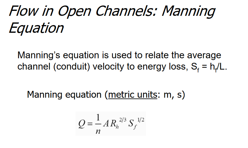
This isn’t quite what we need. It solves for the flow rate (Q), which we already know. And it assumes the channel is sloped (S). Ours has to be horizontal, because it supports flow in both directions, filling and draining.

But I think I can make it work. Suppose I plug in the knowns (or things I can estimate): the flow rate (Q), cross-sectional area (A), hydraulic radius (R), surface roughness (n). Then I could solve for the slope S, but what would be the point when I already know the canal isn’t sloped?

The answer is that S would be the slope of a hypothetical canal, of the same dimensions and materials as ours, which would convey our known flow rate of water, getting just enough energy input along the way to keep up with the frictional losses incurred. And that energy input would come from, of course, gravity: the conversion of gravitational potential energy into kinetic energy due to the water flowing down a slope. So S would tell us the head loss in our real canal per unit length, which is what we want to know.

(The water in our real canal will also become sloped, lower at the draining end—otherwise there’d be nothing driving the flow—even though the canal itself isn’t sloped.)

Converting the Manning formula to solve for S, we get:

   

Before we plug in numbers, let’s look at the relationships. Losses (S) scale as the square of the flow rate (Q), which is true of flow in pipes as well; faster flow makes losses worse, strongly. A is the channel cross-sectional area, and losses scale as the inverse square of that; a bigger channel or pipe makes losses smaller, strongly.

R is the hydraulic radius, which is the the area (A) divided by the wetted perimeter (the total length of the channel’s cross section that is in contact with the flowing water). This wetted perimeter is a bad thing for flow, because the water velocity right at a channel surface is very low due to friction against the non-moving surface. R will have its largest value for a circle, which is the most “compact” shape (least channel surface per unit area). Our trapezoidal channel has lower R, because it has more wetted surface than a circle of the same area. An extremely wide, shallow channel (the opposite of “compact”) would be even worse. As R goes down, losses go up, slightly worse than linearly.

is a roughness parameter, similar to (but not quite the same as) the roughness used for the Darcy-Weisbach formula above. Bigger means rougher (compare finished concrete at 0.012 with gravel at 0.025)⁷. Channels with rougher surfaces lose more energy to friction, which isn’t surprising. So we want the smoothest possible surfaces touching the water. (I would think that since the floating cover does touch the water at all times, it will exert drag on the flow, and so its roughness matters as much as that of the canal sides and bottom.)

Losses in the larger canal design

Now let’s compute an actual value for S. First we need to compute some of the inputs. For the flow rate Q, we might as well use the worst case: the biggest flow we considered above, which was 276 /s. To give our intuition something to chew on, what will the average velocity be? Our channel, at low water, has a cross section (A) of 1,250 ; that leads to an average velocity of 0.22 , about 9 inches a second. That’s a leisurely strolling pace, which is good—slow flow conserves energy.

The wetted perimeter is . So the hydraulic radius R is .

For , I’ll just use the value for concrete, 0.012. Plugging all these numbers in, we get

   

How much slope is that? A canal one kilometer long would have a drop of 0.73 millimeters. That’s utterly negligible, to the point of being a little suspect. There are (at least) three ways to interpret this number:

1. I made a mistake—always a possibility.
   
2. Manning’s equation, which is empirical, is outside its range of applicability here and is giving invalid results⁸.
   
3. The number is correct (within an order of magnitude or two). This would mean that the canal is so large compared to the flow rate that almost no energy is lost to friction.

Losses in the smaller canal design

What about our smaller canal design (still pretty big at 100 meters wide)? Here are the inputs:

flow rate: 276 /s (unchanged)
: 0.012 (unchanged)
area: 200 at lowest allowed water level
Wetted area: 93

Hydraulic radius:

   

This is roughly 2 orders of magnitude (100x) worse than the big canal, due to the much smaller area for water flow. Over a one-kilometer-long canal, the head loss would be 99 millimeters (about 4 inches), which is still negligible. For both canal designs, though we’d certainly want to test a physical or CFD model, energy losses in canals don’t look worrisome.

Transitions

A final place where friction losses are a concern is where the pipes (headraces and tailraces) meet the reservoirs (canals in this case). This is a well-studied topic, and while energy is always lost whenever the flow is disturbed (by a change in direction, a restriction, etc.), the key is to make the change as smoothly and gradually as possible. So the connection at the bottom of a canal should be bell-shaped:

Bends in the headrace, tailrace, and penstock should also be as smooth and gradual as possible.

I’ve done my best to find show-stopping flaws in the hydrodynamics of my plan, but it seems to be holding up so far. In the next post, I’ll apply this design to a real site.

Previous: Encapsulated Pumped Storage, Series 2, Part 1: More Water Containment Options

Next: Encapsulated Pumped Storage, Series 2, Part 3: An Example System

---

1. In 2600 BC, according to this History of Plumbing Timeline
2. Darcy–Weisbach equation (wikipedia)
3. “The Darcy formula or the Darcy-Weisbach equation as it tends to be referred to, is now accepted as the most accurate pipe friction loss formula, and although more difficult to calculate and use than other friction loss formula [sic], with the introduction of computers, it has now become the standard equation for hydraulic engineers.” (https://www.pipeflow.com/pipe-pressure-drop-calculations/pipe-friction-loss)
4. adapted from https://www.pipeflow.com/pipe-pressure-drop-calculations/pipe-friction-loss.
5. https://www.usbr.gov/lc/hooverdam/faqs/tunlfaqs.html
6. It’s really only open-channel flow in a steady state and when far from the outlet. Near the outlet, it’s analogous to drainage from a bathtub, where there is a large downward component to the flow. (As usual, all these phenomena are reversed when water is being pumped into a tank rather than draining out of it.)
7. Unless otherwise stated, values from https://www.caee.utexas.edu/prof/maidment/CE365KSpr14/Visual/OpenChannels.pdf
8. Understanding Open-Channel Flow Equations for Hydro Applications says: “It is known that Manning’s equation loses accuracy with very steep or shallow slopes”